Active learning - part 1

library(knitr)
library(tidyr)
library(dplyr)
library(ggplot2)
library(FSelectorRcpp)
knitr::opts_chunk$set(cache = FALSE, warning = FALSE, message = FALSE, eval = TRUE)

# https://stackoverflow.com/questions/16474696/read-system-tmp-dir-in-r
gettmpdir <- function() {
  tm <- Sys.getenv(c('TMPDIR', 'TMP', 'TEMP'))
  d <- which(file.info(tm)$isdir & file.access(tm, 2) == 0)
  if (length(d) > 0)
    tm[[d[1]]]
  else if (.Platform$OS.type == 'windows')
    Sys.getenv('R_USER')
  else
    '/tmp'
}

dataDir <- file.path(gettmpdir(), "data")
dir.create(dataDir, showWarnings = FALSE, recursive = TRUE)

dataZip <- file.path(dataDir, "bank-data.zip")
dataUrl <- "https://archive.ics.uci.edu/ml/machine-learning-databases/00222/bank.zip"
download.file(dataUrl, dataZip)

unzip(dataZip, exdir = dataDir)

dataPath <- file.path(dataDir, "bank-full.csv")
message("Data path: ", dataPath)

# read data and split into test/traings sets
library(readr)
allData <- readr::read_delim(dataPath, delim = ";", 
  col_types = readr::cols(
  age = col_double(),
  job = col_character(),
  marital = col_character(),
  education = col_character(),
  default = col_character(),
  balance = col_double(),
  housing = col_character(),
  loan = col_character(),
  contact = col_character(),
  day = col_double(),
  month = col_character(),
  duration = col_double(),
  campaign = col_double(),
  pdays = col_double(),
  previous = col_double(),
  poutcome = col_character(),
  y = col_character()
  ))

allData <- allData %>%
  mutate(row_id = row_number()) %>%
  select(-month, -job) %>% # I have a problem with those two columns during 
                           # training phase so I removed them
  mutate(y = y == "yes") # transform to TRUE/FALSE

# split the data into train/test sets.
set.seed(123)
idx <- sample.int(nrow(allData), nrow(allData)*0.2)

trainAll <- allData[-idx,]
testAll <- allData[idx,]

#' @param get_new_idx function which returns the selected rows
#' indexes to be labelled by the oracle. In this function the 'active learning'
#' logic resides.
make_active_learning_path <- function(trainAll, testAll, nstart = 500, n = 50, k = 50, get_new_idx) {

  # init training data set by selecting randomly nstart rows from 
  # 'unlabelled' data
  idxInit <- tibble(row_id = sample(trainAll$row_id, nstart))
  train <- inner_join(trainAll, idxInit, by = "row_id")
  trainAll <- anti_join(trainAll, idxInit, by = "row_id")

  aucRes <- rep(0, n)

  for(i in 1:n) {

    # build a classification model using simple logistics regression
    fit <- glm(y ~ ., data = train %>% select(-row_id), family = "binomial")

    # calculate AUC
    res <- predict(fit, newdata = testAll, type="response")
    aucRes[i] <- suppressMessages(pROC::auc(testAll$y, res, ))

    # select new indexes which will be added to the training set
    newIdx <- get_new_idx(trainAll, train, fit, k)

    trainNew <- inner_join(trainAll, newIdx, by = "row_id")
    train    <- bind_rows(train, trainNew)
    
    # remove selected indexes from available 'unlabelled' set.
    trainAll <- anti_join(trainAll, newIdx,by = "row_id") 
  }
  
  return(aucRes)
}

First experiment - the most uncertain points vs random sample.

In the first attempt I’ll use a function which selects data points for which the model is the most uncertain - in the binary classification task those will be the case where the estimated probability is closest to 0.5:

get_new_idx_most_uncertain <- function(trainAll, train, fit, k) {
    predTrainLeftout <- predict(fit, newdata = trainAll, type="response")
    tr <- trainAll %>% mutate(predTrainLeftout = predTrainLeftout) %>% arrange(abs(predTrainLeftout - 0.5))
    tr %>% select(row_id) %>% head(k)
}

The second function selects the rows at random. There’s nothing fancy in here:

get_new_idx_random <- function(trainAll, train, fit, k) {
  trainAll %>% sample_n(k, replace = FALSE) %>% select(row_id)
}

Let’s run the first two experiments:

# utility function to transform pbreplicate result into data.frame
transform_run <- function(x) {
  xx <- t(x)
  colnames(xx) <- 1:ncol(xx)
  rownames(xx) <- 1:nrow(xx)
  res <- bind_cols(tibble(iter = 1:nrow(xx)), as.data.frame(xx))
  res <- pivot_longer(res, cols = c(-iter), names_to = "round", values_to = "AUC")
  res
}

## performing 20 replications of each simulations
set.seed(123)
mostUncertain <- pbapply::pbreplicate(
  50,
  make_active_learning_path(trainAll, testAll, get_new_idx = get_new_idx_most_uncertain)
  ) %>% transform_run %>% mutate(Type = "1. Most uncertain")

set.seed(123)
allRandom <- pbapply::pbreplicate(
  50,
  make_active_learning_path(trainAll, testAll, get_new_idx = get_new_idx_random)
  ) %>% transform_run %>% mutate(Type = "0. Random")

Some code to visualize the result:

make_plot <- function(result, addRibbon = FALSE) {
  result2 <- result %>% 
    group_by(round, Type) %>%
    summarise(
      AUC_Mean = mean(AUC),
      SD = sd(AUC),
      q025 = quantile(AUC, probs = 0.025),
      q975 = quantile(AUC, probs = 0.975))
  
  p <- ggplot(result2 %>% mutate(round = as.integer(round))) +
    geom_line(aes(round, AUC_Mean, color = Type), size = 1.5) + 
    theme_bw()

  if(addRibbon) {
    p <- p +
      geom_ribbon(aes(round, ymax = q025, ymin = q975, fill = Type), alpha = 0.2)
  }

  return(p)
}

And there it is (each round means additional k samples added to training set, the higher the curve is located the better). Here I was really surprised, because I expected that selecting the points for which the model is the most uncertain would be much better than random sampling, but the opposite is true!

What could be the reason?

make_plot(bind_rows(mostUncertain, allRandom))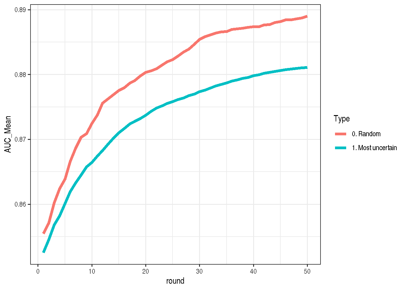

I think for this data set the answer is imbalance in the training data. The most uncertain point is not the 50% but ~11%, because if we would not have any model (and we would just use the percentage of yes answers) we should assume that the probability of yes is around 11%, not 50%.

mean(allData$y)

## [1] 0.1169848

So, let’s adjust the rows selecting function to take care of the class imbalance (the only change is to replace 0.5 with mean(train$y)):

get_new_idx_most_uncertain2 <- function(trainAll, train, fit, k) {
    predTrainLeftout <- predict(fit, newdata = trainAll, type="response")
    tr <- trainAll %>% mutate(predTrainLeftout = predTrainLeftout) %>% arrange(abs(predTrainLeftout - mean(train$y)))
    tr %>% select(row_id) %>% head(k)
}

set.seed(123)
mostUncertain2 <- pbapply::pbreplicate(
  50,
  make_active_learning_path(trainAll, testAll, get_new_idx = get_new_idx_most_uncertain2)
  ) %>% transform_run %>% mutate(Type = "2. Most uncertain - sample based")

As I was expecting, the result looks much better than the first version, but it’s still worse than random selection.

make_plot(bind_rows(mostUncertain, mostUncertain2, allRandom))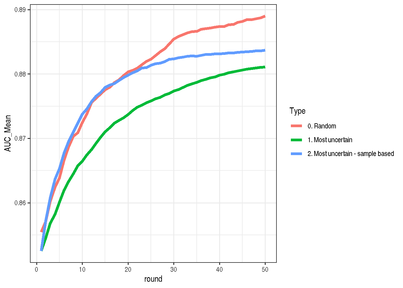

It seems unintuitive, but it makes sense. To score which points should be taken into account I took only raw probability estimates, completely ignoring errors from the model. For one point the estimate might be 26% +- 5% and for another 26% +- 20%. In my case both points are treated equally, which seems wrong. See an example here:

set.seed(123)
fit <- glm(y ~ ., data = trainAll %>% select(-row_id) %>% sample_n(500), family = "binomial")

pred <- predict(fit, se.fit = TRUE)
pred <- tibble(link = pred$fit, se.fit = pred$se.fit) %>% arrange(desc(link))

pred[51:54,] %>%
  mutate(Prob = plogis(link), Prob_1se = plogis(link + se.fit)) %>%
  mutate_all(function(x) round(x, digits = 3)) %>% 
  kable()

link	se.fit	Prob	Prob_1se
-1.161	0.938	0.239	0.445
-1.167	0.679	0.237	0.380
-1.172	0.837	0.236	0.417
-1.178	0.926	0.235	0.437

Some in the next experiment I will select those points where the standard error is the biggest. See the code below:

get_new_idx_most_uncertain3_stdErr_based <- function(trainAll, train, fit, k) {
    stdErr <- predict(fit, newdata = trainAll, se.fit = TRUE)$se.fit
    tr <- trainAll %>% mutate(stdErr = stdErr) %>% arrange(desc(stdErr))
    tr %>% select(row_id) %>% head(k)
}

set.seed(123)
mostUncertain3StdErrBased <- pbapply::pbreplicate(
  50,
  make_active_learning_path(
    trainAll, testAll,
    get_new_idx = get_new_idx_most_uncertain3_stdErr_based)
  ) %>% transform_run %>% mutate(Type = "3. Most uncertain - std.err based")

The idea looked promising, but the reality is tough. This is the worst strategy from all four. Selecting by random is still the best. After some mediation on this result I conclude that this might not be the best idea, because it selects the most noisy points which probably bring much more noise than a good quality signal.

make_plot(bind_rows(mostUncertain, mostUncertain2, allRandom, mostUncertain3StdErrBased))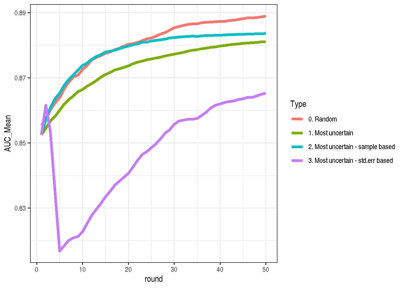

My last idea for now is to remove points with very high standard error. To do this, I’m filtering out everything points with a standard error greater than its 97.5% quantile.

get_new_idx_most_uncertain3_stdErr_trimmed <- function(trainAll, train, fit, k) {
    stdErr <- predict(fit, newdata = trainAll, se.fit = TRUE)$se.fit
    tr <- trainAll %>% mutate(stdErr = stdErr) %>% arrange(desc(stdErr))
    tr <- tr %>% filter(stdErr < quantile(stdErr, probs = 0.975))
    
    tr %>% select(row_id) %>% head(k)
}

set.seed(123)
mostUncertain3StdErrTrimmed <- pbapply::pbreplicate(
  50,
  make_active_learning_path(
    trainAll, testAll,
    get_new_idx = get_new_idx_most_uncertain3_stdErr_trimmed)
  ) %>% transform_run %>% mutate(Type = "4. Most uncertain - std.err trimmed")

Aaand… This is still bad solution. Not as bad as the previous one, but still.

make_plot(
  bind_rows(mostUncertain, mostUncertain2, 
            allRandom, mostUncertain3StdErrBased,
            mostUncertain3StdErrTrimmed))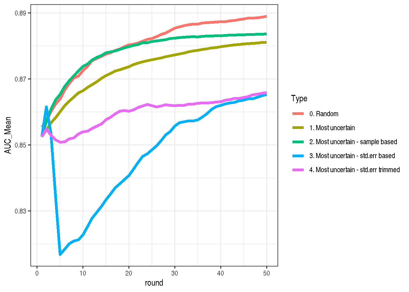

Summary

Active learning is an interesting idea. It’s very exciting that simple and crude solutions do not work very well. It’s really a place where good theory should thrive (or at least be better than random sampling:)). I will probably do a little more experiments in this area to build more intuitions before digging into proper, well-founded methods.