The main purpose of the FSelectorRcpp package is the feature selection based on the entropy function. However, it also contains a function to discretize continuous variable into nominal attributes, and we decided to slightly change the API related to this functionality, to make it more user-friendly.
EDIT: Updated version (0.2.1) is on CRAN. It can be installed using:
install.packages("FSelectorRcpp")The dev version can be installed using devtools:
devtools::install_github("mi2-warsaw/FSelectorRcpp", ref = "dev")discretize now returns all columns by default.
In the current version available on CRAN, calling discretize(Species ~ Sepal.Length, iris return a discretized data frame with only two variables - “Species”, and “Sepal.Length”, all others are discarded. However, it seems to be more natural to return all columns by default, because it allows to easily chain multiple calls to discretize with different methods used for different columns. See the example below:
library(FSelectorRcpp)

# before 0.2.0
discretize(Species ~ Sepal.Length, iris, all = FALSE)
## Species Sepal.Length
## 1 setosa (-Inf,5.55]
## 2 setosa (-Inf,5.55]
## 3 setosa (-Inf,5.55]
## 4 setosa (-Inf,5.55]
## 5 setosa (-Inf,5.55]
## 6 setosa (-Inf,5.55]
## 7 setosa (-Inf,5.55]
## 8 setosa (-Inf,5.55]
## 9 setosa (-Inf,5.55]
## 10 setosa (-Inf,5.55]
## [ reached getOption("max.print") -- omitted 140 rows ]# After - returns all columns by default:
discretize(Species ~ Sepal.Length, iris)## Sepal.Length Sepal.Width Petal.Length Petal.Width Species
## 1 (-Inf,5.55] 3.5 1.4 0.2 setosa
## 2 (-Inf,5.55] 3.0 1.4 0.2 setosa
## 3 (-Inf,5.55] 3.2 1.3 0.2 setosa
## 4 (-Inf,5.55] 3.1 1.5 0.2 setosa
## [ reached getOption("max.print") -- omitted 146 rows ]library(magrittr)
discData <- iris %>%
discretize(Species ~ Sepal.Length, customBreaksControl(c(0, 5, 7.5, 10))) %>%
discretize(Species ~ Sepal.Width, equalsizeControl(5)) %>%
discretize(Species ~ .)
discData## Sepal.Length Sepal.Width Petal.Length Petal.Width Species
## 1 (5,7.5] (3.4, Inf] (-Inf,2.45] (-Inf,0.8] setosa
## 2 (0,5] (3,3.1] (-Inf,2.45] (-Inf,0.8] setosa
## 3 (0,5] (3.1,3.4] (-Inf,2.45] (-Inf,0.8] setosa
## 4 (0,5] (3.1,3.4] (-Inf,2.45] (-Inf,0.8] setosa
## [ reached getOption("max.print") -- omitted 146 rows ]discretize_transform
We also added a discretize_transform which takes a result of the discretize function and uses its cutpoints to discretize new data set. It might be useful in the ML pipelines, where you want to apply the same transformations to the train and test sets.
set.seed(123)
idx <- sort(sample.int(150, 100))
irisTrain <- iris[idx, ]
irisTest <- iris[-idx, ]

discTrain <- irisTrain %>%
  discretize(Species ~ Sepal.Length, customBreaksControl(c(0, 5, 7.5, 10))) %>%
  discretize(Species ~ Sepal.Width, equalsizeControl(5)) %>%
  discretize(Species ~ .)

discTest <- discretize_transform(discTrain, irisTest)

# levels for both columns are equal
all.equal(
  lapply(discTrain, levels),
  lapply(discTest, levels)
)
## [1] TRUEdiscTrain## Sepal.Length Sepal.Width Petal.Length Petal.Width Species
## 1 (5,7.5] (3.4, Inf] (-Inf,2.6] (-Inf,0.8] setosa
## 3 (0,5] (3.2,3.4] (-Inf,2.6] (-Inf,0.8] setosa
## 5 (0,5] (3.4, Inf] (-Inf,2.6] (-Inf,0.8] setosa
## 6 (5,7.5] (3.4, Inf] (-Inf,2.6] (-Inf,0.8] setosa
## [ reached getOption("max.print") -- omitted 96 rows ]discTest## Sepal.Length Sepal.Width Petal.Length Petal.Width Species
## 2 (0,5] (2.75,3] (-Inf,2.6] (-Inf,0.8] setosa
## 4 (0,5] (3,3.2] (-Inf,2.6] (-Inf,0.8] setosa
## 10 (0,5] (3,3.2] (-Inf,2.6] (-Inf,0.8] setosa
## 13 (0,5] (2.75,3] (-Inf,2.6] (-Inf,0.8] setosa
## [ reached getOption("max.print") -- omitted 46 rows ]discretize and information_gain
The code below shows how to compare the feature importance of the two discretization methods applied to the same data. Note that you can discretization using the default method, and then passing the output to the information_gain leads to the same result as directly calling information_gain, on the data without discretization.
library(dplyr)

discTrainCustom <- irisTrain %>%
  discretize(Species ~ Sepal.Length, customBreaksControl(c(0, 5, 7.5, 10))) %>%
  discretize(Species ~ Sepal.Width, equalsizeControl(5)) %>%
  discretize(Species ~ .)

discTrainMdl <- irisTrain %>% discretize(Species ~ .)

custom <- information_gain(Species ~ ., discTrainCustom)
mdl <- information_gain(Species ~ ., discTrainMdl)

all.equal(
  information_gain(Species ~ ., discretize(irisTrain, Species ~ .)),
  information_gain(Species ~ ., discTrainMdl)
)
## [1] TRUEcustom <- custom %>% rename(custom = importance)
mdl <- mdl %>% rename(mdl = importance)
inner_join(mdl, custom, by = "attributes")## attributes mdl custom
## 1 Sepal.Length 0.4340278 0.2368476
## 2 Sepal.Width 0.2333229 0.3301300
## 3 Petal.Length 0.9934589 0.9934589
## 4 Petal.Width 0.9520131 0.9520131customBreaksControl
We also added a new customBreaksControl method, which allows using your breaks in the discretize pipeline. It uses the standard cut function with default arguments, so the output is always closed on the right. If you want more flexibility (like custom labels) feel free to fill an issue on the https://github.com/mi2-warsaw/FSelectorRcpp/issues, and we will see what can be done.
library(ggplot2)
library(tidyr)
library(dplyr)
br <- customBreaksControl(breaks = c(0, 5, 10, Inf))
disc <- discretize(iris, Species ~ ., control = br)

gDisc <- gather(disc, key = "Variable", value = "Value", -Species)

ggplot(gDisc) + geom_bar(aes(Value, fill = Species)) + facet_wrap("Variable")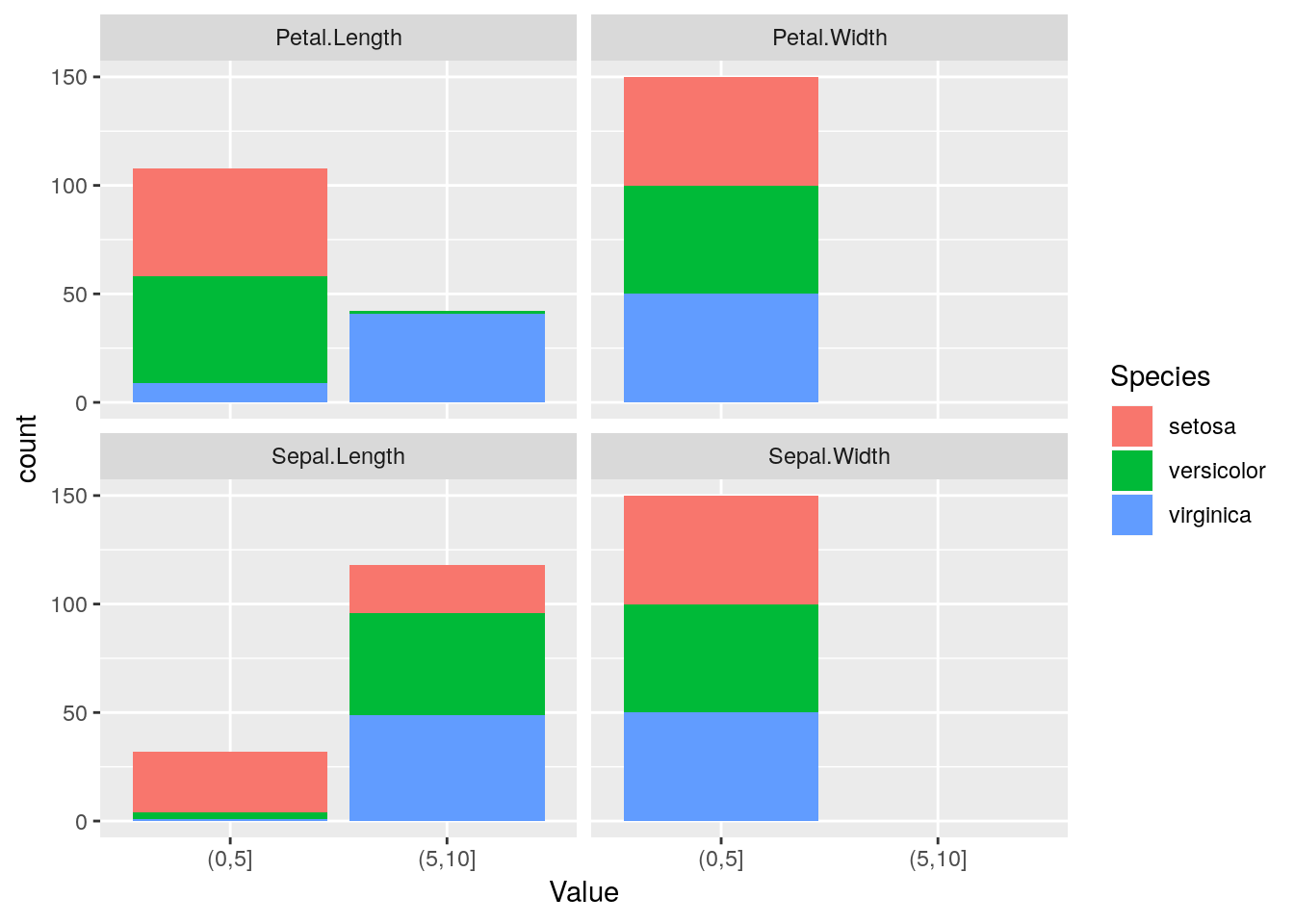
Summary
We still need to do some works on the upcoming release (e.g., write more tests), but we hope you will find it useful.
For more information on FSelectorRcpp you can check:
- http://r-addict.com/2017/01/08/Entropy-Based-Image-Binarization.html
- http://r-addict.com/2017/03/14/FSelectorRcpp-Release.html
- http://r-addict.com/2016/06/19/Venn-Diagram-RTCGA-Feature-Selection.html
- https://cran.r-project.org/web/packages/FSelectorRcpp/vignettes/get_started.html
- https://cran.r-project.org/web/packages/FSelectorRcpp/vignettes/benchmarks_discretize.html