I’m a big fan of Andrew’s Gelman blog (http://andrewgelman.com/). I think that my statistical intuition is way much better after reading it. For example, there’s a post about different types of errors in NHST, not limited to the widely known Type I and Type II errors - http://andrewgelman.com/2004/12/29/type_1_type_2_t/. You should read this before continuing because the rest of this post will be based on it, and the article which is linked in that post (http://www.stat.columbia.edu/~gelman/research/published/francis8.pdf).
The code below performs the simulation described at the beginning of the third paragraph of the “Type S error rates for classical and Bayesian single and multiple comparison procedures” article.
simulation <- function(tau, sigma, n = 2000) {

  # simulate the data as described at the begining of the 3rd paragraph.
  result <- t(replicate(n, {
    dif <- rnorm(n = 1, sd = 2 * tau)
    yy  <- rnorm(1, dif, 2 * sigma)
    c(dif, yy)
  }))

  bThreshold <-
    1.96 * sqrt(2) * sigma * sqrt(1 + (sigma ^ 2) / (tau ^ 2)) # Equation (6)
  clasThreshold <- 1.96 * sqrt(2) * sigma # Equation (5)

  yy <- result[, 2]

  probConfClaimBayes <- mean(yy > bThreshold | yy < -bThreshold)
  probConfClaimClas  <-
    mean(yy > clasThreshold | yy < -clasThreshold)

  bayesConfClaim <- result[yy > bThreshold | yy < -bThreshold,]
  bayesConfClaim <- sign(bayesConfClaim)
  sErrorCondClaimBayes <-
    mean(bayesConfClaim[, 1] != bayesConfClaim[, 2])

  clasConfClaim <-
    result[yy > clasThreshold | yy < -clasThreshold,]
  clasConfClaim <- sign(clasConfClaim)
  sErrorCondClaimClass <-
    mean(clasConfClaim[, 1] != clasConfClaim[, 2])

  list(
    data = result,
    bThreshold = bThreshold,
    clasThreshold = clasThreshold,
    probConfClaimBayes = probConfClaimBayes,
    probConfClaimClas = probConfClaimClas,
    sErrorCondClaimBayes = sErrorCondClaimBayes,
    sErrorCondClaimClass = sErrorCondClaimClass
  )

}

format_result <- function(result) {

  c(
    sprintf("Prob of claim - Bayesian: %.2f%%", result$probConfClaimBayes * 100),
    sprintf("Prob of claim - Classical: %.2f%%", result$probConfClaimClas * 100),
    sprintf("Prob of S-error cond claim - Bayesian: %.2f%%", result$sErrorCondClaimBayes * 100),
    sprintf("Prob of S-error cond claim - Classical: %.2f%%", result$sErrorCondClaimClass * 100))
}

plot_tresholds <- function(result, ...) {
  plot(result$data, xlab = "theta_j - theta_k", ylab = "y_j - y_k", ...)
  abline(h = c(-result$bThreshold, result$bThreshold), lty = 2, col = "green")
  abline(h = c(-result$clasThreshold, result$clasThreshold), lty = 2, col = "red")
  abline(v = 0, lty = 2)
  legend("topleft", c("Bayesian Treshold", "Classical Treshold"), lwd = 2, lty = 1, col = c("green", "red"))

  legend("bottomright", format_result(result))

}
Here you can see the replicated plots from the page 7. I merged the Bayesian and Classical versions into one plot, and I also added the probabilities of claiming that there are differences and the conditional probability of S-Error given the claim.
Note that I got different values than those from figure 3, but the experimental setting might cause it (I’m not using equation described in the test to approximate the result), or I have an error in the code (but I cannot find one…). However, the main point of the article is still valid;)
set.seed(123)
plot_tresholds(simulation(0.5,1,2000), main = "tau: 0.5, sigma: 1")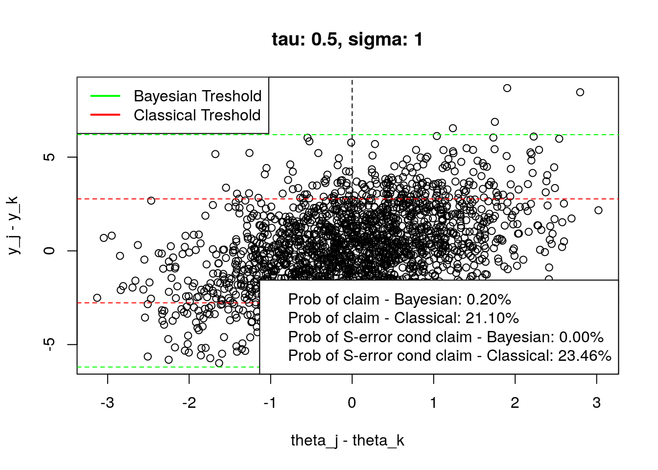
plot_tresholds(simulation(1,1,2000), main = "tau: 1, sigma: 1")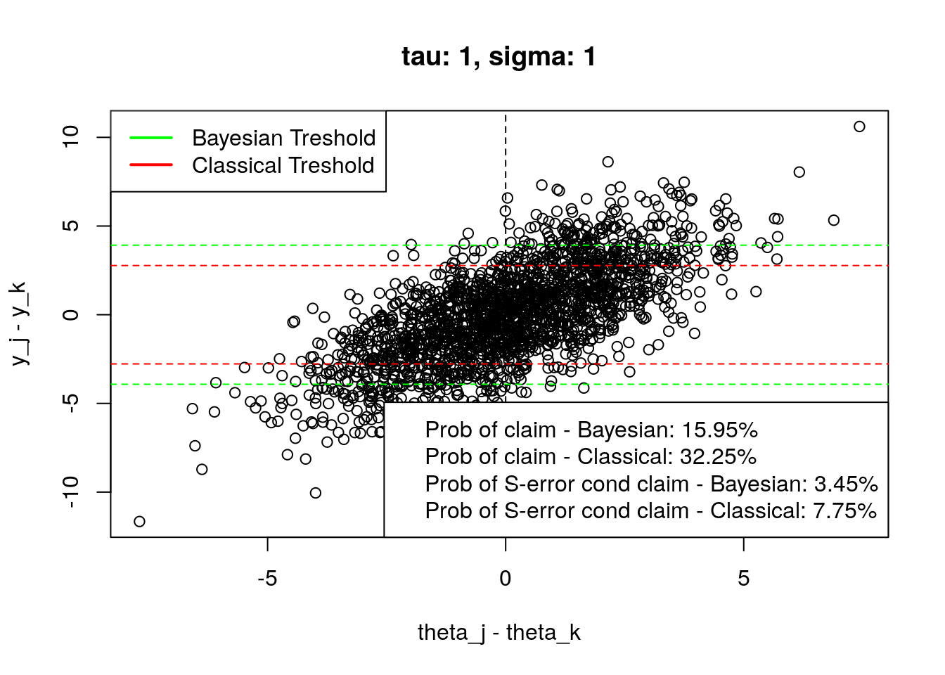
plot_tresholds(simulation(2,1,2000), main = "tau: 2, sigma: 1")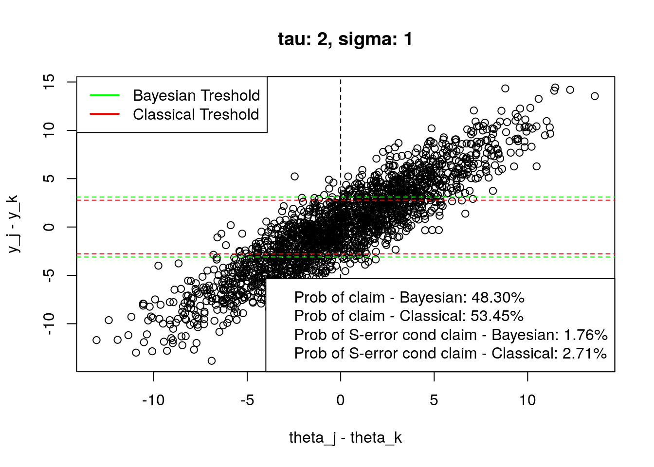
More resources on this topic:
If you want more information about S type errors or related topics check out the links below: